Compared

Tall-cavity natural convection: mean Nusselt number 20 % below the quoted experiment, and refining the grid does not close the gap

I ran wall-resolved k-omega SST on four systematically refined grids of the cavity mid-plane. The grid changes mean Nu by little: the numerical uncertainty is 0.55 %, and the gap to the experimental value is about 47 times that. The gap therefore comes from the model, the inputs, the measurement or the way the experiment defines Nu, and with the data I have I cannot tell which.

Mean Nu, simulation: 4.658; finest of four grids
Mean Nu, experiment: 5.85; quoted second-hand (KBwiki UFR 4-10)
Signed difference: −20.4 %; simulation minus experiment
Numerical uncertainty: ±0.025; least squares on four grids, 95 %

Case: ERCOFTAC C-079, tall differentially heated air cavity
Solver: OpenFOAM v2412, buoyantSimpleFoam
Turbulence model: k-omega SST, resolved to the wall
Cells: 8,000 to 64,410 (four grids)
Rayleigh number: 0.86 × 10⁶ (cavity width)
Status: Compared
Updated: 2026-11-14

2Geometry, mesh, results

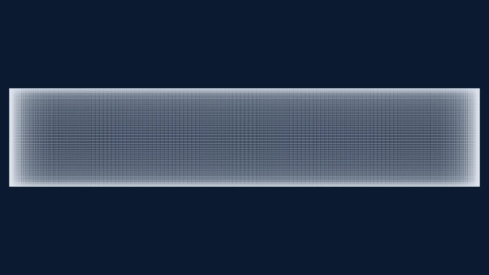
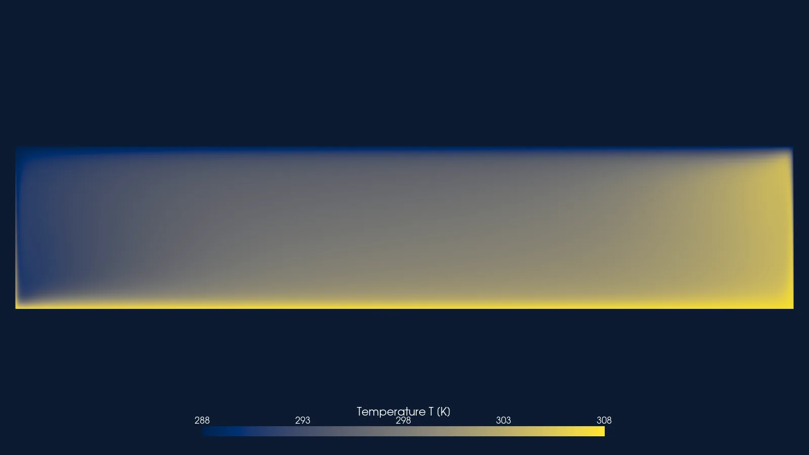
Tall air-filled cavity, 2-D section: heated and cooled side walls, top and bottom walls held at the measured temperature profile; walls drawn as lines. Not to scale: the cavity is 28.7 times taller than wide, so its width is drawn 6 times true scale and it is turned on its side (hot wall at the bottom, top end at the right); probe positions are in true coordinates.

Not to scale: x drawn 6 times true scale. Probe positions are given in true coordinates.

3Case parameters

Rayleigh number (cavity width)	0.86 × 10⁶
Height, width, depth	2.18 m, 0.076 m, 0.52 m
Wall temperatures	307.75 K and 288.15 K (19.6 K)
Fluid	Air, Pr 0.705
Solver	OpenFOAM v2412, buoyantSimpleFoam
Turbulence model	k-omega SST, wall-resolved
Wall y+ max	0.097 finest, 0.26 coarsest
Cells	8,000 to 64,410
Fluid properties	perfect gas, constant properties: Cp 1004.4 J/kg K, viscosity 1.831e-05 Pa s, molar mass 28.96 kg/kmol
Gravity	(0 −9.81 0) m/s²
Run cost	Not recorded

4Experiment

Betts and Bokhari built an air-filled cavity 2.18 m high, 0.076 m wide and 0.52 m deep, with isothermal aluminium side walls 19.6 K apart and 5 cm hard rubber, k = 0.155 W/mK top and bottom walls with thermocouples at mid-thickness. Velocity was measured by laser-Doppler velocimetry and temperature with a traversed thermocouple. The source describes the flow on the mid-plane as closely two-dimensional.

The open ERCOFTAC files give mean temperature and mean vertical velocity across the cavity at 9 heights (y/H 0.05 to 0.95), temperature normal to the floor and roof at x = 38.1 mm, and the temperature inside the rubber walls, which I used as boundary conditions. The mean Nusselt number 5.85 is not in those files: it is quoted on the ERCOFTAC KBwiki page UFR 4-10, without its definition.

One file has a defect: at y/H 0.10, four points at x = 40.6–55.8 mm alternate 4–5 K above their neighbours. They are plotted as given.

Stated uncertainty	Not stated in the source. The experimental uncertainty and the experiment's definition of the mean Nusselt number are on neither open page; the journal paper is closed access and I have not read it.
Blockage and corrections	Not applicable: a closed cavity, no tunnel.
Licence	ERCOFTAC Classic Collection case 079 (University of Manchester), data of Betts and Bokhari, CC BY-NC-SA 4.0. The tables and CSV files here are derived from that data and carry the same licence.

Mean temperature at y/H 0.5 (x in mm, T in °C)

Experimental values (51 points)

x from the cold wall (mm)	Experiment (Betts and Bokhari)
0.33	15.62
0.58	15.94
0.84	16.45
1.09	16.78
1.6	17.58
2.11	18.48
2.61	19.05
3.25	19.43
3.88	19.96
5.15	20.46
6.42	21.32
7.69	21.74
8.96	22.01
10.23	22.21
11.5	22.53
12.77	22.74
15.31	23.02
17.85	23.35
20.39	23.76
22.93	23.69
25.47	24.17
28.01	24.25
30.55	25.08
33.09	25.15
35.63	25.33
38.17	25.26
40.57	25.23
43.11	25.57
45.65	25.92
48.19	26.12
50.73	25.87
53.27	26.3
55.81	26.55
58.35	26.99
60.89	27.05
63.43	27.53
64.7	27.65
65.97	27.77
67.24	27.71
68.51	28.38
69.78	28.61
71.05	29.44
72.32	30.06
72.95	30.5
73.59	31.12
74.09	31.66
74.6	32.37
75.11	33.08
75.36	33.37
75.62	33.94
75.87	34.21

Download CSV

Mean vertical velocity at y/H 0.5 (x in mm, V in m/s)

Experimental values (28 points)

x from the cold wall (mm)	Experiment (Betts and Bokhari)
1.2	-0.081
2.2	-0.115
3.2	-0.124
4.2	-0.133
6.2	-0.135
8.2	-0.134
10.2	-0.12
12.2	-0.112
14.2	-0.11
16.2	-0.1
18.2	-0.089
23.2	-0.062
28.2	-0.048
33.2	-0.011
38.2	0.012
43.2	0.041
48.2	0.054
53.2	0.077
58.2	0.091
60.2	0.099
62.2	0.106
64.2	0.12
66.2	0.127
68.2	0.133
70.2	0.137
71.2	0.14
72.2	0.131
73.2	0.121

Download CSV

5Set-up

A 2-D slice of the cavity mid-plane, 2.18 m by 0.076 m, one cell (0.01 m) thick with empty front and back faces. The parent case is the stock buoyantCavity tutorial (3-D, wall functions, adiabatic top and bottom). I changed three things on purpose: the 2-D slice, wall-resolved SST, and top and bottom walls held at the measured rubber-wall temperature instead of adiabatic.

The cavity is closed, so there is no inlet or outlet: the flow is driven by the 19.6 K between the side walls. Values below are from the finest grid's 0/ files; the other grids use the same recipe.

Boundary conditions
Boundary	Type	Value
Hot wall (x = W)	no-slip; fixed temperature	307.75 K
Cold wall (x = 0)	no-slip; fixed temperature	288.15 K
Bottom and top walls	no-slip; fixed temperature, one value per face	non-uniform list of measured values (the rubber-wall temperature profile)
All four walls, turbulence	k fixed; omega omegaWallFunction; nut nutLowReWallFunction; alphat compressible::alphatWallFunction	k 1e-12 m²/s²; turbulent Prandtl number 0.85
All four walls, pressure	fixedFluxPressure (p_rgh)	1e5 Pa
Front and back	empty (2-D)

Numerics and convergence

Steady buoyantSimpleFoam with gravity (0 −9.81 0) m/s², initial temperature 297.95 K. Convection terms for U, energy and turbulence: bounded Gauss limitedLinear 0.2. Pressure relaxation 0.7.

Convergence was judged from the Nusselt-number history. The finest grid was extended from 20,000 to 35,000 iterations because Nu was still drifting in one direction. At the end, the hot-wall Nu varies by 2.17e-05 (relative) over the last 2000 iterations, and the heat balance over all walls closes to 7 × 10⁻⁵ of the wall flux.

The Nusselt number is my definition, Nu = q_mean W / (k ΔT), with W the cavity width and k from Cp, viscosity and Prandtl number. On the finest grid the hot wall gives 4.6607 and the cold wall 4.6551; the page uses their mean.

6Mesh

Cells, finest grid	64,410
Structure	One block, 114 × 565 cells, graded towards every wall
y+ max, finest grid (cold wall)	0.097
Max non-orthogonality	0
Max skewness	1.2e-11
Max aspect ratio	80
checkMesh verdict, finest grid	“Mesh OK.”

The four grids, same recipe, grid-size ratio about 1.41 between neighbours. Mean Nu and the signed difference from the quoted 5.85 are as written by compare.py for each grid.
Grid	Cells	Iterations	Mean Nu	vs experiment	checkMesh
g0.5 (coarsest)	8,000	20,000	4.5962	−21.43 %	“Mesh OK.”
g0.7071	15,848	20,000	4.6262	−20.92 %	“Mesh OK.”
g1.0	32,000	20,000	4.6459	−20.58 %	“Mesh OK.”
g1.4142 (finest)	64,410	35,000	4.6579	−20.38 %	“Mesh OK.”

Every grid passed checkMesh; the log of each exact mesh was read before it was solved. The mesh is a single orthogonal block, so non-orthogonality is zero and skewness is at round-off level.

7Results

On the finest of four grids the mean Nusselt number is 4.658 ±0.025, against 5.85 quoted for the experiment: −20.4 %.

Mean Nusselt number on the four grids (4.5962 on 8,000 cells to 4.6579 on 64,410), the least-squares extrapolation 4.678, and the experimental 5.85 as a dashed reference line. The grid moves Nu by a small fraction of the gap.

Data table (4 rows)

Cells	Simulation, k-omega SST	Least-squares extrapolation	Experiment (quoted, KBwiki UFR 4-10)
8000	4.5962	4.678092	5.85
15848	4.6262	4.678092	5.85
32000	4.6459	4.678092	5.85
64410	4.6579	4.678092	5.85

Download CSV

Mean temperature across the cavity at mid-height, y/H 0.5. RMS difference 0.513 K. Simulation values converted to the experiment's units in one place (pipeline/case_data/betts-bokhari-cavity.py), the same conversion compare.py uses: x [mm] = 1000 × x [m], T [°C] = T [K] − 273.15.

Data tables, one per series (51 points, 400 points)

Experiment (Betts and Bokhari)
x from the cold wall (mm)	Experiment (Betts and Bokhari)
0.33	15.62
0.58	15.94
0.84	16.45
1.09	16.78
1.6	17.58
2.11	18.48
2.61	19.05
3.25	19.43
3.88	19.96
5.15	20.46
6.42	21.32
7.69	21.74
8.96	22.01
10.23	22.21
11.5	22.53
12.77	22.74
15.31	23.02
17.85	23.35
20.39	23.76
22.93	23.69
25.47	24.17
28.01	24.25
30.55	25.08
33.09	25.15
35.63	25.33
38.17	25.26
40.57	25.23
43.11	25.57
45.65	25.92
48.19	26.12
50.73	25.87
53.27	26.3
55.81	26.55
58.35	26.99
60.89	27.05
63.43	27.53
64.7	27.65
65.97	27.77
67.24	27.71
68.51	28.38
69.78	28.61
71.05	29.44
72.32	30.06
72.95	30.5
73.59	31.12
74.09	31.66
74.6	32.37
75.11	33.08
75.36	33.37
75.62	33.94
75.87	34.21

Simulation, finest grid
x from the cold wall (mm)	Simulation, finest grid
0	15
0.19047619	15.21713
0.38095238	15.43368
0.57142857	15.65103
0.76190476	15.86871
0.95238095	16.08389
1.1428571	16.30177
1.3333333	16.51896
1.5238095	16.73444
1.7142857	16.94998
1.9047619	17.16543
2.0952381	17.38057
2.2857143	17.59512
2.4761905	17.80871
2.6666667	18.02061
2.8571429	18.22754
3.047619	18.43167
3.2380952	18.63535
3.4285714	18.83408
3.6190476	19.02481
3.8095238	19.21273
4	19.39312
4.1904762	19.56593
4.3809524	19.73302
4.5714286	19.88984
4.7619048	20.03991
4.952381	20.18111
5.1428571	20.31474
5.3333333	20.44073
5.5238095	20.55903
5.7142857	20.67083
5.9047619	20.77486
6.0952381	20.87337
6.2857143	20.96598
6.4761905	21.05355
6.6666667	21.13685
6.8571429	21.21532
7.047619	21.28917
7.2380952	21.35938
7.4285714	21.42642
7.6190476	21.4908
7.8095238	21.55104
8	21.60914
8.1904762	21.66546
8.3809524	21.71822
8.5714286	21.76938
8.7619048	21.81903
8.952381	21.86599
9.1428571	21.91183
9.3333333	21.9558
9.5238095	21.99831
9.7142857	22.03996
9.9047619	22.07931
10.095238	22.11824
10.285714	22.15558
10.47619	22.19218
10.666667	22.22731
10.857143	22.26183
11.047619	22.2955
11.238095	22.32816
11.428571	22.35984
11.619048	22.39097
11.809524	22.4215
12	22.45124
12.190476	22.47996
12.380952	22.50844
12.571429	22.53627
12.761905	22.56391
12.952381	22.5901
13.142857	22.61628
13.333333	22.64191
13.52381	22.66741
13.714286	22.69212
13.904762	22.71612
14.095238	22.74007
14.285714	22.76355
14.47619	22.78704
14.666667	22.80963
14.857143	22.83172
15.047619	22.8538
15.238095	22.87553
15.428571	22.89726
15.619048	22.9184
15.809524	22.93884
16	22.95929
16.190476	22.97956
16.380952	22.99976
16.571429	23.01996
16.761905	23.03903
16.952381	23.05804
17.142857	23.07704
17.333333	23.09591
17.52381	23.11477
17.714286	23.13354
17.904762	23.15129
18.095238	23.16904
18.285714	23.1868
18.47619	23.2045
18.666667	23.22221
18.857143	23.23991
19.047619	23.25671
19.238095	23.27337
19.428571	23.29003
19.619048	23.30679
19.809524	23.32363
20	23.34047
20.190476	23.35706
20.380952	23.37291
20.571429	23.38876
20.761905	23.40461
20.952381	23.42085
21.142857	23.43723
21.333333	23.45362
21.52381	23.46978
21.714286	23.4852
21.904762	23.50062
22.095238	23.51604
22.285714	23.53183
22.47619	23.54799
22.666667	23.56414
22.857143	23.5803
23.047619	23.59574
23.238095	23.61095
23.428571	23.62616
23.619048	23.64137
23.809524	23.65716
24	23.6731
24.190476	23.68904
24.380952	23.70497
24.571429	23.72014
24.761905	23.73515
24.952381	23.75015
25.142857	23.76516
25.333333	23.78057
25.52381	23.79622
25.714286	23.81187
25.904762	23.82752
26.095238	23.84281
26.285714	23.85755
26.47619	23.87229
26.666667	23.88704
26.857143	23.90178
27.047619	23.91704
27.238095	23.93235
27.428571	23.94766
27.619048	23.96297
27.809524	23.97789
28	23.99231
28.190476	24.00674
28.380952	24.02116
28.571429	24.03558
28.761905	24.05036
28.952381	24.06531
29.142857	24.08026
29.333333	24.09521
29.52381	24.11016
29.714286	24.12431
29.904762	24.1384
30.095238	24.15249
30.285714	24.16657
30.47619	24.18066
30.666667	24.1952
30.857143	24.20982
31.047619	24.22443
31.238095	24.23905
31.428571	24.25366
31.619048	24.2676
31.809524	24.28138
32	24.29515
32.190476	24.30892
32.380952	24.3227
32.571429	24.33672
32.761905	24.35107
32.952381	24.36541
33.142857	24.37975
33.333333	24.3941
33.52381	24.40839
33.714286	24.42192
33.904762	24.43544
34.095238	24.44896
34.285714	24.46249
34.47619	24.47601
34.666667	24.48976
34.857143	24.50392
35.047619	24.51809
35.238095	24.53225
35.428571	24.54642
35.619048	24.56058
35.809524	24.57423
36	24.58759
36.190476	24.60095
36.380952	24.61431
36.571429	24.62767
36.761905	24.64103
36.952381	24.65458
37.142857	24.66827
37.333333	24.68196
37.52381	24.69566
37.714286	24.70935
37.904762	24.72304
38.095238	24.73674
38.285714	24.75043
38.47619	24.76412
38.666667	24.77782
38.857143	24.79151
39.047619	24.8052
39.238095	24.81876
39.428571	24.83213
39.619048	24.84551
39.809524	24.85888
40	24.87226
40.190476	24.88564
40.380952	24.8993
40.571429	24.91349
40.761905	24.92767
40.952381	24.94186
41.142857	24.95604
41.333333	24.97022
41.52381	24.984
41.714286	24.99755
41.904762	25.01111
42.095238	25.02466
42.285714	25.03822
42.47619	25.05178
42.666667	25.06611
42.857143	25.08049
43.047619	25.09486
43.238095	25.10924
43.428571	25.12362
43.619048	25.13769
43.809524	25.15151
44	25.16533
44.190476	25.17915
44.380952	25.19298
44.571429	25.20696
44.761905	25.22163
44.952381	25.2363
45.142857	25.25096
45.333333	25.26563
45.52381	25.28022
45.714286	25.29437
45.904762	25.30852
46.095238	25.32267
46.285714	25.33682
46.47619	25.35104
46.666667	25.36605
46.857143	25.38107
47.047619	25.39609
47.238095	25.4111
47.428571	25.42595
47.619048	25.44045
47.809524	25.45495
48	25.46945
48.190476	25.48395
48.380952	25.49895
48.571429	25.51434
48.761905	25.52973
48.952381	25.54512
49.142857	25.56047
49.333333	25.5753
49.52381	25.59013
49.714286	25.60496
49.904762	25.61979
50.095238	25.63517
50.285714	25.65092
50.47619	25.66667
50.666667	25.68241
50.857143	25.69791
51.047619	25.71302
51.238095	25.72813
51.428571	25.74324
51.619048	25.7585
51.809524	25.77455
52	25.79059
52.190476	25.80664
52.380952	25.82253
52.571429	25.83786
52.761905	25.85318
52.952381	25.86851
53.142857	25.88406
53.333333	25.90034
53.52381	25.91661
53.714286	25.93289
53.904762	25.9488
54.095238	25.96436
54.285714	25.97991
54.47619	25.99547
54.666667	26.01177
54.857143	26.02829
55.047619	26.04481
55.238095	26.06121
55.428571	26.07723
55.619048	26.09325
55.809524	26.10927
56	26.12604
56.190476	26.14306
56.380952	26.16009
56.571429	26.17705
56.761905	26.19392
56.952381	26.2108
57.142857	26.22782
57.333333	26.24575
57.52381	26.26369
57.714286	26.28162
57.904762	26.29963
58.095238	26.31764
58.285714	26.33565
58.47619	26.35468
58.666667	26.37382
58.857143	26.39295
59.047619	26.41226
59.238095	26.43156
59.428571	26.45093
59.619048	26.47145
59.809524	26.49197
60	26.51256
60.190476	26.53336
60.380952	26.55415
60.571429	26.57566
60.761905	26.59776
60.952381	26.61986
61.142857	26.64235
61.333333	26.66485
61.52381	26.68787
61.714286	26.71179
61.904762	26.73571
62.095238	26.76014
62.285714	26.78462
62.47619	26.80984
62.666667	26.83586
62.857143	26.86201
63.047619	26.88877
63.238095	26.91553
63.428571	26.94378
63.619048	26.97223
63.809524	27.00137
64	27.03078
64.190476	27.06123
64.380952	27.09248
64.571429	27.1244
64.761905	27.15689
64.952381	27.1904
65.142857	27.22494
65.333333	27.26039
65.52381	27.29651
65.714286	27.33413
65.904762	27.37252
66.095238	27.41263
66.285714	27.45316
66.47619	27.49607
66.666667	27.53991
66.857143	27.58532
67.047619	27.63266
67.238095	27.68118
67.428571	27.73257
67.619048	27.78553
67.809524	27.84015
68	27.8986
68.190476	27.95888
68.380952	28.0214
68.571429	28.08836
68.761905	28.15809
68.952381	28.23115
69.142857	28.3081
69.333333	28.38987
69.52381	28.47673
69.714286	28.56808
69.904762	28.66468
70.095238	28.76744
70.285714	28.87595
70.47619	28.99241
70.666667	29.11563
70.857143	29.2465
71.047619	29.38526
71.238095	29.53131
71.428571	29.68643
71.619048	29.84766
71.809524	30.01925
72	30.19584
72.190476	30.3797
72.380952	30.57068
72.571429	30.76371
72.761905	30.96444
72.952381	31.16971
73.142857	31.37484
73.333333	31.58248
73.52381	31.79483
73.714286	32.00862
73.904762	32.22318
74.095238	32.4382
74.285714	32.65341
74.47619	32.86865
74.666667	33.08379
74.857143	33.30061
75.047619	33.5181
75.238095	33.73289
75.428571	33.95018
75.619048	34.16712
75.809524	34.38327
76	34.6

Download CSV

Mean vertical velocity across the cavity at mid-height, y/H 0.5: upward next to the hot wall, downward next to the cold wall. Peak up and peak down, experiment then simulation: 0.140 and 0.166 m/s; −0.135 and −0.165 m/s. Velocities are in m/s in both files; x converted as x [mm] = 1000 × x [m].

Data tables, one per series (28 points, 400 points)

Experiment (Betts and Bokhari)
x from the cold wall (mm)	Experiment (Betts and Bokhari)
1.2	-0.081
2.2	-0.115
3.2	-0.124
4.2	-0.133
6.2	-0.135
8.2	-0.134
10.2	-0.12
12.2	-0.112
14.2	-0.11
16.2	-0.1
18.2	-0.089
23.2	-0.062
28.2	-0.048
33.2	-0.011
38.2	0.012
43.2	0.041
48.2	0.054
53.2	0.077
58.2	0.091
60.2	0.099
62.2	0.106
64.2	0.12
66.2	0.127
68.2	0.133
70.2	0.137
71.2	0.14
72.2	0.131
73.2	0.121

Simulation, finest grid
x from the cold wall (mm)	Simulation, finest grid
0	0
0.19047619	-0.01422819
0.38095238	-0.027666972
0.57142857	-0.040404305
0.76190476	-0.052442119
0.95238095	-0.063690923
1.1428571	-0.074342633
1.3333333	-0.084315504
1.5238095	-0.093588311
1.7142857	-0.10224261
1.9047619	-0.11027611
2.0952381	-0.11769064
2.2857143	-0.12449322
2.4761905	-0.13069746
2.6666667	-0.13631731
2.8571429	-0.14132332
3.047619	-0.14583334
3.2380952	-0.14968719
3.4285714	-0.15305235
3.6190476	-0.15597194
3.8095238	-0.15830435
4	-0.1602388
4.1904762	-0.16182647
4.3809524	-0.16292278
4.5714286	-0.1638498
4.7619048	-0.16430148
4.952381	-0.16467191
5.1428571	-0.16468708
5.3333333	-0.16466332
5.5238095	-0.16434958
5.7142857	-0.16405316
5.9047619	-0.16351084
6.0952381	-0.16298771
6.2857143	-0.16233741
6.4761905	-0.16164635
6.6666667	-0.16093888
6.8571429	-0.16012068
7.047619	-0.15935074
7.2380952	-0.15850318
7.4285714	-0.15763556
7.6190476	-0.15680231
7.8095238	-0.15588253
8	-0.15498444
8.1904762	-0.15411152
8.3809524	-0.15316198
8.5714286	-0.15224128
8.7619048	-0.15134774
8.952381	-0.15039199
9.1428571	-0.14944922
9.3333333	-0.14854471
9.5238095	-0.14760188
9.7142857	-0.1466365
9.9047619	-0.14572433
10.095238	-0.14480832
10.285714	-0.14384342
10.47619	-0.14289744
10.666667	-0.14198941
10.857143	-0.14105893
11.047619	-0.14009732
11.238095	-0.1391643
11.428571	-0.13825933
11.619048	-0.13732993
11.809524	-0.13637313
12	-0.13544097
12.190476	-0.13454049
12.380952	-0.13362596
12.571429	-0.13267463
12.761905	-0.13172976
12.952381	-0.1308344
13.142857	-0.12993904
13.333333	-0.12900237
13.52381	-0.12805657
13.714286	-0.12713983
13.904762	-0.12624965
14.095238	-0.12535529
14.285714	-0.12441465
14.47619	-0.123474
14.666667	-0.12256886
14.857143	-0.12168348
15.047619	-0.12079559
15.238095	-0.11985941
15.428571	-0.11892323
15.619048	-0.11801214
15.809524	-0.11713092
16	-0.11624969
16.190476	-0.11533241
16.380952	-0.11439976
16.571429	-0.11346712
16.761905	-0.11258619
16.952381	-0.11170824
17.142857	-0.11082934
17.333333	-0.10989908
17.52381	-0.10896882
17.714286	-0.10804346
17.904762	-0.10716769
18.095238	-0.10629192
18.285714	-0.10541614
18.47619	-0.10448807
18.666667	-0.10355887
18.857143	-0.10262968
19.047619	-0.10174763
19.238095	-0.10087278
19.428571	-0.099997932
19.619048	-0.099087611
19.809524	-0.098149603
20	-0.097211595
20.190476	-0.096287589
20.380952	-0.095404359
20.571429	-0.094521128
20.761905	-0.093637898
20.952381	-0.092693342
21.142857	-0.091727528
21.333333	-0.090761714
21.52381	-0.089808824
21.714286	-0.088899312
21.904762	-0.0879898
22.095238	-0.087080288
22.285714	-0.086123451
22.47619	-0.085118628
22.666667	-0.084113805
22.857143	-0.083108982
23.047619	-0.082148797
23.238095	-0.081202437
23.428571	-0.080256077
23.619048	-0.079309717
23.809524	-0.078287494
24	-0.07724592
24.190476	-0.076204346
24.380952	-0.075162772
24.571429	-0.074171388
24.761905	-0.073190285
24.952381	-0.072209181
25.142857	-0.071228077
25.333333	-0.07019218
25.52381	-0.06912196
25.714286	-0.068051739
25.904762	-0.066981519
26.095238	-0.065936073
26.285714	-0.064927836
26.47619	-0.063919599
26.666667	-0.062911361
26.857143	-0.061903124
27.047619	-0.060819771
27.238095	-0.059729938
27.428571	-0.058640105
27.619048	-0.057550273
27.809524	-0.056488231
28	-0.055461347
28.190476	-0.054434462
28.380952	-0.053407577
28.571429	-0.052380693
28.761905	-0.051302619
28.952381	-0.050200669
29.142857	-0.049098718
29.333333	-0.047996768
29.52381	-0.046894818
29.714286	-0.045851395
29.904762	-0.0448129
30.095238	-0.043774405
30.285714	-0.04273591
30.47619	-0.041697415
30.666667	-0.040598125
30.857143	-0.039489326
31.047619	-0.038380526
31.238095	-0.037271727
31.428571	-0.036162928
31.619048	-0.03510549
31.809524	-0.034060323
32	-0.033015157
32.190476	-0.031969991
32.380952	-0.030924825
32.571429	-0.029850585
32.761905	-0.028738248
32.952381	-0.027625912
33.142857	-0.026513575
33.333333	-0.025401238
33.52381	-0.024292624
33.714286	-0.02324388
33.904762	-0.022195136
34.095238	-0.021146393
34.285714	-0.020097649
34.47619	-0.019048905
34.666667	-0.017977499
34.857143	-0.016863577
35.047619	-0.015749655
35.238095	-0.014635733
35.428571	-0.01352181
35.619048	-0.012407888
35.809524	-0.011334351
36	-0.010283842
36.190476	-0.0092333318
36.380952	-0.008182822
36.571429	-0.0071323122
36.761905	-0.0060818024
36.952381	-0.0050134603
37.142857	-0.0039315794
37.333333	-0.0028496985
37.52381	-0.0017678175
37.714286	-0.00068593663
37.904762	0.00039594429
38.095238	0.0014778291
38.285714	0.0025597179
38.47619	0.0036416067
38.666667	0.0047234954
38.857143	0.0058053842
39.047619	0.006887273
39.238095	0.0079557461
39.428571	0.0090065491
39.619048	0.010057352
39.809524	0.011108155
40	0.012158958
40.190476	0.013209761
40.380952	0.014283603
40.571429	0.015397851
40.761905	0.016512099
40.952381	0.017626346
41.142857	0.018740594
41.333333	0.019854842
41.52381	0.020926668
41.714286	0.021975882
41.904762	0.023025096
42.095238	0.024074309
42.285714	0.025123523
42.47619	0.026172737
42.666667	0.02728186
42.857143	0.028394708
43.047619	0.029507555
43.238095	0.030620403
43.428571	0.03173325
43.619048	0.032808053
43.809524	0.033853822
44	0.034899591
44.190476	0.03594536
44.380952	0.036991129
44.571429	0.03804918
44.761905	0.039158629
44.952381	0.040268078
45.142857	0.041377528
45.333333	0.042486977
45.52381	0.043586919
45.714286	0.044626076
45.904762	0.045665234
46.095238	0.046704391
46.285714	0.047743548
46.47619	0.048787637
46.666667	0.0498903
46.857143	0.050992963
47.047619	0.052095626
47.238095	0.05319829
47.428571	0.054277045
47.619048	0.055304546
47.809524	0.056332046
48	0.057359546
48.190476	0.058387046
48.380952	0.05944973
48.571429	0.060540227
48.761905	0.061630724
48.952381	0.062721221
49.142857	0.063805221
49.333333	0.064813907
49.52381	0.065822593
49.714286	0.066831278
49.904762	0.067839964
50.095238	0.068885882
50.285714	0.069956589
50.47619	0.071027297
50.666667	0.072098005
50.857143	0.07313428
51.047619	0.074115588
51.238095	0.075096896
51.428571	0.076078204
51.619048	0.077069796
51.809524	0.078111599
52	0.079153402
52.190476	0.080195204
52.380952	0.081217618
52.571429	0.082164021
52.761905	0.083110423
52.952381	0.084056825
53.142857	0.085017055
53.333333	0.086021934
53.52381	0.087026814
53.714286	0.088031693
53.904762	0.088988706
54.095238	0.08989851
54.285714	0.090808315
54.47619	0.091718119
54.666667	0.092671324
54.857143	0.093637459
55.047619	0.094603595
55.238095	0.095548782
55.428571	0.096433534
55.619048	0.097318286
55.809524	0.098203038
56	0.099128642
56.190476	0.10006827
56.380952	0.10100791
56.571429	0.10192027
56.761905	0.10279771
56.952381	0.10367514
57.142857	0.1045598
57.333333	0.10549175
57.52381	0.1064237
57.714286	0.10735452
57.904762	0.10823316
58.095238	0.10911179
58.285714	0.10999043
58.47619	0.11091881
58.666667	0.11185211
58.857143	0.11278542
59.047619	0.11366746
59.238095	0.11454857
59.428571	0.11543265
59.619048	0.11636864
59.809524	0.11730463
60	0.11822528
60.190476	0.11910995
60.380952	0.11999461
60.571429	0.12090926
60.761905	0.12184908
60.952381	0.12278891
61.142857	0.12368052
61.333333	0.12456962
61.52381	0.12547858
61.714286	0.12642317
61.904762	0.12736776
62.095238	0.12826611
62.285714	0.1291603
62.47619	0.13008115
62.666667	0.13103119
62.857143	0.1319721
63.047619	0.1328717
63.238095	0.1337713
63.428571	0.13472064
63.619048	0.13567647
63.809524	0.13659545
64	0.13750036
64.190476	0.13843709
64.380952	0.13939859
64.571429	0.14033258
64.761905	0.14124206
64.952381	0.14217971
65.142857	0.14314611
65.333333	0.14408114
65.52381	0.14499358
65.714286	0.14594414
65.904762	0.14691371
66.095238	0.14783381
66.285714	0.14875
66.47619	0.14971962
66.666667	0.15066628
66.857143	0.1515739
67.047619	0.15251992
67.238095	0.15347882
67.428571	0.1543738
67.619048	0.155296
67.809524	0.15624707
68	0.1571186
68.190476	0.15801519
68.380952	0.1589331
68.571429	0.15976012
68.761905	0.16062125
68.952381	0.16145982
69.142857	0.16221593
69.333333	0.16301944
69.52381	0.16370419
69.714286	0.16436904
69.904762	0.16498749
70.095238	0.16546807
70.285714	0.16596492
70.47619	0.16619665
70.666667	0.16644197
70.857143	0.1663763
71.047619	0.16626414
71.238095	0.16577542
71.428571	0.16519547
71.619048	0.1641207
71.809524	0.16286523
72	0.16110699
72.190476	0.1589953
72.380952	0.15647918
72.571429	0.15338177
72.761905	0.14983865
72.952381	0.14581238
73.142857	0.14114918
73.333333	0.13600242
73.52381	0.13025545
73.714286	0.12394219
73.904762	0.11705065
74.095238	0.10956843
74.285714	0.10148936
74.47619	0.09281222
74.666667	0.083539753
74.857143	0.073591074
75.047619	0.06298892
75.238095	0.051818491
75.428571	0.039887586
75.619048	0.027288248
75.809524	0.014020853
76	1.3589325e-14

Download CSV

Mean temperature near the floor, y/H 0.10. Hollow markers: four points of the ERCOFTAC file mt_z0_10_lo.dat, at x = 40.57, 45.65, 50.73 and 55.81 mm, that sit 4–5 K above their neighbours and match the mid-height values of mt_z0_40_lo.dat and mt_z0_50_lo.dat at the same x; the file header does not explain them and the cause upstream is not determined. They are shown as published, not deleted or moved. The RMS difference copied from the run's RESULT.txt, 1.448 K, includes them; without them it is 0.32 K. Units converted as x [mm] = 1000 × x [m], T [°C] = T [K] − 273.15.

Data tables, one per series (47 points, 4 points, 400 points)

Experiment (Betts and Bokhari)
x from the cold wall (mm)	Experiment (Betts and Bokhari)
0.33	15.13
0.58	15.38
0.84	15.65
1.09	15.82
1.6	16.29
2.11	16.72
2.61	17.15
3.25	17.44
3.88	17.79
5.15	18.37
6.42	18.72
7.69	19.04
8.96	19.14
10.23	19.57
11.5	19.62
12.77	19.8
15.31	20.02
17.85	20.23
20.39	20.46
22.93	20.48
25.47	20.48
28.01	20.67
30.55	20.69
33.09	20.71
35.63	20.87
38.17	20.79
43.11	20.73
48.19	20.87
53.27	20.93
58.35	21.25
60.89	21.29
63.43	21.72
64.7	21.77
65.97	22.52
67.24	23.09
68.51	23.87
69.78	24.99
71.05	26.42
72.32	28.32
72.95	29.14
73.59	30.1
74.09	31.15
74.6	32.06
75.11	33.15
75.36	33.52
75.62	33.99
75.87	34.6

Experiment, as published, suspect (4 points)
x from the cold wall (mm)	Experiment, as published, suspect (4 points)
40.57	24.66
45.65	25.36
50.73	25.62
55.81	26.09

Simulation, finest grid
x from the cold wall (mm)	Simulation, finest grid
0	15
0.19047619	15.1138
0.38095238	15.22693
0.57142857	15.34004
0.76190476	15.45313
0.95238095	15.56619
1.1428571	15.67919
1.3333333	15.79212
1.5238095	15.90493
1.7142857	16.0176
1.9047619	16.13008
2.0952381	16.24233
2.2857143	16.35428
2.4761905	16.46589
2.6666667	16.57708
2.8571429	16.68763
3.047619	16.79753
3.2380952	16.90677
3.4285714	17.01521
3.6190476	17.12225
3.8095238	17.2284
4	17.33316
4.1904762	17.43601
4.3809524	17.53806
4.5714286	17.63672
4.7619048	17.73473
4.952381	17.82888
5.1428571	17.92217
5.3333333	18.01095
5.5238095	18.09927
5.7142857	18.18175
5.9047619	18.26424
6.0952381	18.3407
6.2857143	18.41616
6.4761905	18.48787
6.6666667	18.55587
6.8571429	18.62386
7.047619	18.68433
7.2380952	18.7448
7.4285714	18.80279
7.6190476	18.85601
7.8095238	18.90923
8	18.95899
8.1904762	19.0055
8.3809524	19.052
8.5714286	19.0954
8.7619048	19.13587
8.952381	19.17633
9.1428571	19.21506
9.3333333	19.25019
9.5238095	19.28532
9.7142857	19.32045
9.9047619	19.35124
10.095238	19.38172
10.285714	19.4122
10.47619	19.44134
10.666667	19.46779
10.857143	19.49425
11.047619	19.5207
11.238095	19.54539
11.428571	19.56836
11.619048	19.59133
11.809524	19.6143
12	19.63595
12.190476	19.65591
12.380952	19.67587
12.571429	19.69582
12.761905	19.71548
12.952381	19.73282
13.142857	19.75016
13.333333	19.7675
13.52381	19.78484
13.714286	19.80098
13.904762	19.81604
14.095238	19.8311
14.285714	19.84616
14.47619	19.86122
14.666667	19.875
14.857143	19.88807
15.047619	19.90113
15.238095	19.91419
15.428571	19.92726
15.619048	19.93952
15.809524	19.95083
16	19.96214
16.190476	19.97345
16.380952	19.98475
16.571429	19.99606
16.761905	20.0059
16.952381	20.01566
17.142857	20.02542
17.333333	20.03517
17.52381	20.04493
17.714286	20.05456
17.904762	20.06294
18.095238	20.07132
18.285714	20.0797
18.47619	20.08807
18.666667	20.09645
18.857143	20.10483
19.047619	20.11214
19.238095	20.11929
19.428571	20.12644
19.619048	20.13359
19.809524	20.14074
20	20.14789
20.190476	20.15476
20.380952	20.1608
20.571429	20.16685
20.761905	20.1729
20.952381	20.17895
21.142857	20.185
21.333333	20.19105
21.52381	20.19687
21.714286	20.20193
21.904762	20.207
22.095238	20.21206
22.285714	20.21712
22.47619	20.22218
22.666667	20.22725
22.857143	20.23231
23.047619	20.23669
23.238095	20.24087
23.428571	20.24504
23.619048	20.24922
23.809524	20.25339
24	20.25757
24.190476	20.26174
24.380952	20.26592
24.571429	20.26943
24.761905	20.27281
24.952381	20.27619
25.142857	20.27956
25.333333	20.28294
25.52381	20.28632
25.714286	20.2897
25.904762	20.29307
26.095238	20.29616
26.285714	20.29883
26.47619	20.30149
26.666667	20.30415
26.857143	20.30681
27.047619	20.30948
27.238095	20.31214
27.428571	20.3148
27.619048	20.31746
27.809524	20.31984
28	20.32187
28.190476	20.32389
28.380952	20.32592
28.571429	20.32794
28.761905	20.32997
28.952381	20.33199
29.142857	20.33402
29.333333	20.33604
29.52381	20.33807
29.714286	20.33957
29.904762	20.34103
30.095238	20.3425
30.285714	20.34396
30.47619	20.34542
30.666667	20.34688
30.857143	20.34834
31.047619	20.34981
31.238095	20.35127
31.428571	20.35273
31.619048	20.3538
31.809524	20.35478
32	20.35575
32.190476	20.35673
32.380952	20.3577
32.571429	20.35868
32.761905	20.35966
32.952381	20.36063
33.142857	20.36161
33.333333	20.36258
33.52381	20.36354
33.714286	20.36411
33.904762	20.36468
34.095238	20.36525
34.285714	20.36582
34.47619	20.36639
34.666667	20.36696
34.857143	20.36753
35.047619	20.3681
35.238095	20.36867
35.428571	20.36924
35.619048	20.36981
35.809524	20.37018
36	20.37043
36.190476	20.37069
36.380952	20.37094
36.571429	20.37119
36.761905	20.37145
36.952381	20.3717
37.142857	20.37196
37.333333	20.37221
37.52381	20.37246
37.714286	20.37272
37.904762	20.37297
38.095238	20.37313
38.285714	20.37318
38.47619	20.37324
38.666667	20.37329
38.857143	20.37335
39.047619	20.3734
39.238095	20.37346
39.428571	20.37351
39.619048	20.37357
39.809524	20.37362
40	20.37368
40.190476	20.37373
40.380952	20.37376
40.571429	20.37374
40.761905	20.37371
40.952381	20.37369
41.142857	20.37367
41.333333	20.37365
41.52381	20.37362
41.714286	20.3736
41.904762	20.37358
42.095238	20.37355
42.285714	20.37353
42.47619	20.37351
42.666667	20.37353
42.857143	20.37355
43.047619	20.37357
43.238095	20.37359
43.428571	20.37361
43.619048	20.37364
43.809524	20.37366
44	20.37368
44.190476	20.3737
44.380952	20.37372
44.571429	20.37377
44.761905	20.37396
44.952381	20.37415
45.142857	20.37434
45.333333	20.37453
45.52381	20.37471
45.714286	20.3749
45.904762	20.37509
46.095238	20.37528
46.285714	20.37546
46.47619	20.37567
46.666667	20.37616
46.857143	20.37664
47.047619	20.37712
47.238095	20.37761
47.428571	20.37809
47.619048	20.37857
47.809524	20.37906
48	20.37954
48.190476	20.38002
48.380952	20.38075
48.571429	20.38167
48.761905	20.38259
48.952381	20.38351
49.142857	20.38443
49.333333	20.38535
49.52381	20.38627
49.714286	20.38719
49.904762	20.38811
50.095238	20.38939
50.285714	20.3909
50.47619	20.39242
50.666667	20.39393
50.857143	20.39544
51.047619	20.39696
51.238095	20.39847
51.428571	20.39999
51.619048	20.40163
51.809524	20.40394
52	20.40624
52.190476	20.40854
52.380952	20.41085
52.571429	20.41315
52.761905	20.41545
52.952381	20.41776
53.142857	20.42031
53.333333	20.42368
53.52381	20.42705
53.714286	20.43041
53.904762	20.43378
54.095238	20.43715
54.285714	20.44051
54.47619	20.44388
54.666667	20.44836
54.857143	20.45318
55.047619	20.458
55.238095	20.46281
55.428571	20.46763
55.619048	20.47245
55.809524	20.47726
56	20.48355
56.190476	20.49033
56.380952	20.49711
56.571429	20.5039
56.761905	20.51068
56.952381	20.51746
57.142857	20.5246
57.333333	20.53401
57.52381	20.54343
57.714286	20.55284
57.904762	20.56226
58.095238	20.57168
58.285714	20.58109
58.47619	20.59366
58.666667	20.60654
58.857143	20.61942
59.047619	20.6323
59.238095	20.64518
59.428571	20.6583
59.619048	20.67564
59.809524	20.69297
60	20.71031
60.190476	20.72765
60.380952	20.74499
60.571429	20.76538
60.761905	20.78832
60.952381	20.81127
61.142857	20.83422
61.333333	20.85716
61.52381	20.88257
61.714286	20.9124
61.904762	20.94222
62.095238	20.97205
62.285714	21.00187
62.47619	21.03563
62.666667	21.07369
62.857143	21.11175
63.047619	21.1498
63.238095	21.18786
63.428571	21.23443
63.619048	21.2821
63.809524	21.32978
64	21.37746
64.190476	21.43131
64.380952	21.48996
64.571429	21.54862
64.761905	21.60728
64.952381	21.672
65.142857	21.74291
65.333333	21.81383
65.52381	21.88474
65.714286	21.96459
65.904762	22.04889
66.095238	22.13319
66.285714	22.21841
66.47619	22.31699
66.666667	22.41556
66.857143	22.51413
67.047619	22.62273
67.238095	22.73615
67.428571	22.84958
67.619048	22.97029
67.809524	23.09873
68	23.22717
68.190476	23.36276
68.380952	23.50601
68.571429	23.64925
68.761905	23.80248
68.952381	23.9609
69.142857	24.11931
69.333333	24.29511
69.52381	24.47092
69.714286	24.65679
69.904762	24.85285
70.095238	25.05196
70.285714	25.26949
70.47619	25.48702
70.666667	25.72406
70.857143	25.96265
71.047619	26.21775
71.238095	26.47597
71.428571	26.74944
71.619048	27.02549
71.809524	27.3157
72	27.60941
72.190476	27.91152
72.380952	28.21986
72.571429	28.53229
72.761905	28.85124
72.952381	29.17405
73.142857	29.50013
73.333333	29.82938
73.52381	30.16202
73.714286	30.49686
73.904762	30.83361
74.095238	31.17201
74.285714	31.51179
74.47619	31.85267
74.666667	32.19442
74.857143	32.5369
75.047619	32.87988
75.238095	33.22319
75.428571	33.56675
75.619048	33.91044
75.809524	34.25419
76	34.6

Download CSV

Mean vertical velocity near the floor, y/H 0.1. Peak up and peak down, experiment then simulation: 0.193 and 0.178 m/s; −0.101 and −0.112 m/s. x converted as x [mm] = 1000 × x [m].

Data tables, one per series (30 points, 400 points)

Experiment (Betts and Bokhari)
x from the cold wall (mm)	Experiment (Betts and Bokhari)
1.5	-0.049
3.5	-0.086
5.5	-0.095
7.5	-0.101
9.5	-0.098
10.5	-0.096
12.5	-0.087
14.5	-0.081
16.5	-0.078
18.5	-0.07
20.5	-0.064
25.5	-0.052
30.5	-0.044
35.5	-0.028
38.2	-0.019
43.2	-0.011
48.2	0.003
53.2	0.023
58.2	0.038
60.2	0.055
62.2	0.07
64.2	0.09
66.2	0.121
68.2	0.151
69.2	0.168
70.2	0.18
71.2	0.19
72.2	0.192
73.2	0.193
74.2	0.16

Simulation, finest grid
x from the cold wall (mm)	Simulation, finest grid
0	0
0.19047619	-0.0083134831
0.38095238	-0.016200619
0.57142857	-0.023717271
0.76190476	-0.030877057
0.95238095	-0.037655682
1.1428571	-0.044108373
1.3333333	-0.050219162
1.5238095	-0.05597451
1.7142857	-0.061410779
1.9047619	-0.066530121
2.0952381	-0.071337537
2.2857143	-0.075841262
2.4761905	-0.080053175
2.6666667	-0.083980196
2.8571429	-0.087554363
3.047619	-0.09085976
3.2380952	-0.093922052
3.4285714	-0.096724199
3.6190476	-0.099175147
3.8095238	-0.10143956
4	-0.10343608
4.1904762	-0.1051431
4.3809524	-0.10672955
4.5714286	-0.10792311
4.7619048	-0.10905624
4.952381	-0.10984542
5.1428571	-0.11057673
5.3333333	-0.11100157
5.5238095	-0.11140257
5.7142857	-0.11150342
5.9047619	-0.11160427
6.0952381	-0.11147077
6.2857143	-0.11129837
6.4761905	-0.11101684
6.6666667	-0.11062749
6.8571429	-0.11023798
7.047619	-0.10968728
7.2380952	-0.10913659
7.4285714	-0.10854745
7.6190476	-0.10788442
7.8095238	-0.10722139
8	-0.10652078
8.1904762	-0.10578507
8.3809524	-0.10504935
8.5714286	-0.10429161
8.7619048	-0.10351312
8.952381	-0.10273463
9.1428571	-0.10194921
9.3333333	-0.10114935
9.5238095	-0.10034949
9.7142857	-0.09954963
9.9047619	-0.098743573
10.095238	-0.097937085
10.285714	-0.097130596
10.47619	-0.096325184
10.666667	-0.095521929
10.857143	-0.094718675
11.047619	-0.093915421
11.238095	-0.093117056
11.428571	-0.092323485
11.619048	-0.091529914
11.809524	-0.090736343
12	-0.089948812
12.190476	-0.089169045
12.380952	-0.088389279
12.571429	-0.087609512
12.761905	-0.086831634
12.952381	-0.086068232
13.142857	-0.08530483
13.333333	-0.084541428
13.52381	-0.083778026
13.714286	-0.083023975
13.904762	-0.082278462
14.095238	-0.08153295
14.285714	-0.080787438
14.47619	-0.080041925
14.666667	-0.079308447
14.857143	-0.07858167
15.047619	-0.077854892
15.238095	-0.077128115
15.428571	-0.076401337
15.619048	-0.075683294
15.809524	-0.074975654
16	-0.074268013
16.190476	-0.073560372
16.380952	-0.072852732
16.571429	-0.072145091
16.761905	-0.07145566
16.952381	-0.070767272
17.142857	-0.070078885
17.333333	-0.069390498
17.52381	-0.068702111
17.714286	-0.068015451
17.904762	-0.067346253
18.095238	-0.066677054
18.285714	-0.066007855
18.47619	-0.065338657
18.666667	-0.064669458
18.857143	-0.06400026
19.047619	-0.063347555
19.238095	-0.062697367
19.428571	-0.062047179
19.619048	-0.06139699
19.809524	-0.060746802
20	-0.060096614
20.190476	-0.059451221
20.380952	-0.058819793
20.571429	-0.058188366
20.761905	-0.057556939
20.952381	-0.056925511
21.142857	-0.056294084
21.333333	-0.055662656
21.52381	-0.055035468
21.714286	-0.054422506
21.904762	-0.053809543
22.095238	-0.053196581
22.285714	-0.052583619
22.47619	-0.051970657
22.666667	-0.051357695
22.857143	-0.050744733
23.047619	-0.050145617
23.238095	-0.049550789
23.428571	-0.048955961
23.619048	-0.048361133
23.809524	-0.047766305
24	-0.047171477
24.190476	-0.046576648
24.380952	-0.04598182
24.571429	-0.045401738
24.761905	-0.044824677
24.952381	-0.044247615
25.142857	-0.043670553
25.333333	-0.043093491
25.52381	-0.042516429
25.714286	-0.041939367
25.904762	-0.041362305
26.095238	-0.040792177
26.285714	-0.040232463
26.47619	-0.039672749
26.666667	-0.039113034
26.857143	-0.03855332
27.047619	-0.037993605
27.238095	-0.037433891
27.428571	-0.036874177
27.619048	-0.036314462
27.809524	-0.035762189
28	-0.03521933
28.190476	-0.03467647
28.380952	-0.034133611
28.571429	-0.033590752
28.761905	-0.033047892
28.952381	-0.032505033
29.142857	-0.031962173
29.333333	-0.031419314
29.52381	-0.030876455
29.714286	-0.030348588
29.904762	-0.029821984
30.095238	-0.029295379
30.285714	-0.028768775
30.47619	-0.02824217
30.666667	-0.027715566
30.857143	-0.027188962
31.047619	-0.026662357
31.238095	-0.026135753
31.428571	-0.025609148
31.619048	-0.025095033
31.809524	-0.024583902
32	-0.02407277
32.190476	-0.023561639
32.380952	-0.023050508
32.571429	-0.022539376
32.761905	-0.022028245
32.952381	-0.021517114
33.142857	-0.021005983
33.333333	-0.020494851
33.52381	-0.01998456
33.714286	-0.01948777
33.904762	-0.01899098
34.095238	-0.018494191
34.285714	-0.017997401
34.47619	-0.017500612
34.666667	-0.017003822
34.857143	-0.016507033
35.047619	-0.016010243
35.238095	-0.015513453
35.428571	-0.015016664
35.619048	-0.014519874
35.809524	-0.014035704
36	-0.01355873
36.190476	-0.013081756
36.380952	-0.012604782
36.571429	-0.012127807
36.761905	-0.011650833
36.952381	-0.011173859
37.142857	-0.010696884
37.333333	-0.01021991
37.52381	-0.0097429359
37.714286	-0.0092659616
37.904762	-0.0087889874
38.095238	-0.008316811
38.285714	-0.0078494325
38.47619	-0.0073820539
38.666667	-0.0069146754
38.857143	-0.0064472969
39.047619	-0.0059799184
39.238095	-0.0055125399
39.428571	-0.0050451614
39.619048	-0.0045777829
39.809524	-0.0041104044
40	-0.0036430259
40.190476	-0.0031756474
40.380952	-0.002710411
40.571429	-0.0022489315
40.761905	-0.0017874521
40.952381	-0.0013259726
41.142857	-0.00086449312
41.333333	-0.00040301365
41.52381	0.000058465826
41.714286	0.0005199453
41.904762	0.00098142477
42.095238	0.0014429042
42.285714	0.0019043837
42.47619	0.0023658632
42.666667	0.0028249171
42.857143	0.0032838202
43.047619	0.0037427233
43.238095	0.0042016265
43.428571	0.0046605296
43.619048	0.0051194327
43.809524	0.0055783358
44	0.0060372389
44.190476	0.006496142
44.380952	0.0069550452
44.571429	0.0074158355
44.761905	0.0078845237
44.952381	0.008353212
45.142857	0.0088219002
45.333333	0.0092905884
45.52381	0.0097592767
45.714286	0.010227965
45.904762	0.010696653
46.095238	0.011165341
46.285714	0.01163403
46.47619	0.012103312
46.666667	0.012579652
46.857143	0.013055992
47.047619	0.013532332
47.238095	0.014008672
47.428571	0.014485012
47.619048	0.014961352
47.809524	0.015437691
48	0.015914031
48.190476	0.016390371
48.380952	0.01687395
48.571429	0.017363252
48.761905	0.017852554
48.952381	0.018341856
49.142857	0.018831158
49.333333	0.01932046
49.52381	0.019809762
49.714286	0.020299063
49.904762	0.020788365
50.095238	0.021288933
50.285714	0.021797003
50.47619	0.022305072
50.666667	0.022813141
50.857143	0.023321211
51.047619	0.02382928
51.238095	0.024337349
51.428571	0.024845419
51.619048	0.025358127
51.809524	0.025893481
52	0.026428835
52.190476	0.02696419
52.380952	0.027499544
52.571429	0.028034899
52.761905	0.028570253
52.952381	0.029105608
53.142857	0.029650848
53.333333	0.030228007
53.52381	0.030805167
53.714286	0.031382326
53.904762	0.031959486
54.095238	0.032536645
54.285714	0.033113805
54.47619	0.033690964
54.666667	0.034315406
54.857143	0.034953934
55.047619	0.035592463
55.238095	0.036230992
55.428571	0.036869521
55.619048	0.03750805
55.809524	0.038146579
56	0.038846856
56.190476	0.039568338
56.380952	0.040289819
56.571429	0.041011301
56.761905	0.041732782
56.952381	0.042454264
57.142857	0.04318974
57.333333	0.04401696
57.52381	0.04484418
57.714286	0.0456714
57.904762	0.046498619
58.095238	0.047325839
58.285714	0.048153059
58.47619	0.049098052
58.666667	0.050054699
58.857143	0.051011346
59.047619	0.051967993
59.238095	0.052924641
59.428571	0.053889585
59.619048	0.054999229
59.809524	0.056108873
60	0.057218518
60.190476	0.058328162
60.380952	0.059437806
60.571429	0.060642549
60.761905	0.061927143
60.952381	0.063211737
61.142857	0.064496331
61.333333	0.065780925
61.52381	0.067134736
61.714286	0.068612859
61.904762	0.070090983
62.095238	0.071569107
62.285714	0.073047231
62.47619	0.07462411
62.666667	0.076309128
62.857143	0.077994146
63.047619	0.079679163
63.238095	0.081364181
63.428571	0.083237825
63.619048	0.08513608
63.809524	0.087034335
64	0.088932591
64.190476	0.09094948
64.380952	0.093058647
64.571429	0.095167814
64.761905	0.097276981
64.952381	0.099484377
65.142857	0.10179196
65.333333	0.10409954
65.52381	0.10640712
65.714286	0.10883101
65.904762	0.11131289
66.095238	0.11379476
66.285714	0.11628559
66.47619	0.11890489
66.666667	0.12152419
66.857143	0.12414349
67.047619	0.12682172
67.238095	0.12952828
67.428571	0.13223484
67.619048	0.13495313
67.809524	0.13768388
68	0.14041463
68.190476	0.14312213
68.380952	0.14580474
68.571429	0.14848735
68.761905	0.15109888
68.952381	0.15367343
69.142857	0.15624798
69.333333	0.15868297
69.52381	0.16111781
69.714286	0.16346307
69.904762	0.16571764
70.095238	0.1679342
70.285714	0.16992176
70.47619	0.17190932
70.666667	0.17353949
70.857143	0.17514128
71.047619	0.17631122
71.238095	0.1773996
71.428571	0.1779293
71.619048	0.1783583
71.809524	0.17807221
72	0.1775455
72.190476	0.17644101
72.380952	0.17476191
72.571429	0.17267707
72.761905	0.16979724
72.952381	0.16630211
73.142857	0.1622221
73.333333	0.15748276
73.52381	0.15185331
73.714286	0.14548797
73.904762	0.13835733
74.095238	0.13041867
74.285714	0.12163907
74.47619	0.11199521
74.666667	0.10147286
74.857143	0.089963564
75.047619	0.077498507
75.238095	0.064117848
75.428571	0.04966249
75.619048	0.034198264
75.809524	0.017685368
76	1.7235025e-14

Download CSV

Mean temperature near the roof, y/H 0.9. RMS difference 0.662 K. Units converted as x [mm] = 1000 × x [m], T [°C] = T [K] − 273.15.

Data tables, one per series (51 points, 400 points)

Experiment (Betts and Bokhari)
x from the cold wall (mm)	Experiment (Betts and Bokhari)
0.33	15.61
0.58	16.32
0.84	16.8
1.09	17.38
1.6	18.36
2.11	19.52
2.61	20.39
3.25	21.64
3.88	22.49
5.15	24.23
6.42	25.68
7.69	26.84
8.96	27.48
10.23	28.1
11.5	28.55
12.77	28.97
15.31	29.26
17.85	29.52
20.39	29.53
22.93	29.54
25.47	29.55
28.01	29.6
30.55	29.67
33.09	29.71
35.63	29.74
38.17	29.73
40.57	29.93
43.11	29.99
45.65	30.07
48.19	30.1
50.73	30.12
53.27	30.18
55.81	30.29
58.35	30.4
60.89	30.57
63.43	30.69
64.7	30.85
65.97	31.02
67.24	31.19
68.51	31.48
69.78	31.68
71.05	32.06
72.32	32.52
72.95	32.77
73.59	33.2
74.09	33.49
74.6	33.78
75.11	34.19
75.36	34.38
75.62	34.6
75.87	34.77

Simulation, finest grid
x from the cold wall (mm)	Simulation, finest grid
0	15
0.19047619	15.3444
0.38095238	15.68674
0.57142857	16.02902
0.76190476	16.37117
0.95238095	16.71305
1.1428571	17.05459
1.3333333	17.39562
1.5238095	17.73588
1.7142857	18.07524
1.9047619	18.41344
2.0952381	18.7502
2.2857143	19.08524
2.4761905	19.41827
2.6666667	19.749
2.8571429	20.07617
3.047619	20.4
3.2380952	20.72039
3.4285714	21.03671
3.6190476	21.34618
3.8095238	21.65134
4	21.94998
4.1904762	22.23984
4.3809524	22.52605
4.5714286	22.79759
4.7619048	23.06648
4.952381	23.31974
5.1428571	23.56984
5.3333333	23.8032
5.5238095	24.03501
5.7142857	24.24727
5.9047619	24.45953
6.0952381	24.65352
6.2857143	24.84447
6.4761905	25.02534
6.6666667	25.19625
6.8571429	25.36715
7.047619	25.52088
7.2380952	25.67461
7.4285714	25.8233
7.6190476	25.9623
7.8095238	26.10129
8	26.23294
8.1904762	26.35773
8.3809524	26.48252
8.5714286	26.59988
8.7619048	26.71025
8.952381	26.82062
9.1428571	26.92636
9.3333333	27.02246
9.5238095	27.11856
9.7142857	27.21466
9.9047619	27.29791
10.095238	27.38027
10.285714	27.46263
10.47619	27.5407
10.666667	27.61016
10.857143	27.67962
11.047619	27.74908
11.238095	27.81257
11.428571	27.87021
11.619048	27.92784
11.809524	27.98548
12	28.03847
12.190476	28.08549
12.380952	28.13251
12.571429	28.17954
12.761905	28.22548
12.952381	28.2632
13.142857	28.30091
13.333333	28.33862
13.52381	28.37633
13.714286	28.40987
13.904762	28.4396
14.095238	28.46932
14.285714	28.49905
14.47619	28.52877
14.666667	28.5542
14.857143	28.57723
15.047619	28.60026
15.238095	28.62329
15.428571	28.64632
15.619048	28.66685
15.809524	28.68441
16	28.70196
16.190476	28.71951
16.380952	28.73706
16.571429	28.75462
16.761905	28.76803
16.952381	28.7812
17.142857	28.79437
17.333333	28.80754
17.52381	28.82071
17.714286	28.83358
17.904762	28.84333
18.095238	28.85307
18.285714	28.86282
18.47619	28.87257
18.666667	28.88232
18.857143	28.89206
19.047619	28.89953
19.238095	28.90665
19.428571	28.91378
19.619048	28.9209
19.809524	28.92802
20	28.93514
20.190476	28.94175
20.380952	28.94689
20.571429	28.95203
20.761905	28.95717
20.952381	28.96231
21.142857	28.96745
21.333333	28.97259
21.52381	28.97739
21.714286	28.98105
21.904762	28.98471
22.095238	28.98837
22.285714	28.99203
22.47619	28.99569
22.666667	28.99935
22.857143	29.00301
23.047619	29.00583
23.238095	29.00839
23.428571	29.01096
23.619048	29.01352
23.809524	29.01609
24	29.01865
24.190476	29.02121
24.380952	29.02378
24.571429	29.02567
24.761905	29.02742
24.952381	29.02917
25.142857	29.03092
25.333333	29.03267
25.52381	29.03442
25.714286	29.03618
25.904762	29.03793
26.095238	29.03944
26.285714	29.04058
26.47619	29.04172
26.666667	29.04286
26.857143	29.04401
27.047619	29.04515
27.238095	29.04629
27.428571	29.04744
27.619048	29.04858
27.809524	29.04953
28	29.05022
28.190476	29.05092
28.380952	29.05161
28.571429	29.05231
28.761905	29.05301
28.952381	29.0537
29.142857	29.0544
29.333333	29.0551
29.52381	29.05579
29.714286	29.05621
29.904762	29.0566
30.095238	29.05699
30.285714	29.05738
30.47619	29.05778
30.666667	29.05817
30.857143	29.05856
31.047619	29.05895
31.238095	29.05934
31.428571	29.05974
31.619048	29.05999
31.809524	29.06021
32	29.06043
32.190476	29.06065
32.380952	29.06087
32.571429	29.06109
32.761905	29.06131
32.952381	29.06152
33.142857	29.06174
33.333333	29.06196
33.52381	29.06218
33.714286	29.06235
33.904762	29.06253
34.095238	29.0627
34.285714	29.06287
34.47619	29.06305
34.666667	29.06322
34.857143	29.06339
35.047619	29.06356
35.238095	29.06374
35.428571	29.06391
35.619048	29.06408
35.809524	29.06431
36	29.06456
36.190476	29.06481
36.380952	29.06506
36.571429	29.06531
36.761905	29.06556
36.952381	29.06581
37.142857	29.06607
37.333333	29.06632
37.52381	29.06657
37.714286	29.06682
37.904762	29.06707
38.095238	29.06743
38.285714	29.06788
38.47619	29.06834
38.666667	29.0688
38.857143	29.06926
39.047619	29.06972
39.238095	29.07017
39.428571	29.07063
39.619048	29.07109
39.809524	29.07155
40	29.07201
40.190476	29.07246
40.380952	29.07304
40.571429	29.07383
40.761905	29.07462
40.952381	29.07541
41.142857	29.0762
41.333333	29.07699
41.52381	29.07778
41.714286	29.07857
41.904762	29.07936
42.095238	29.08015
42.285714	29.08094
42.47619	29.08172
42.666667	29.08291
42.857143	29.08412
43.047619	29.08533
43.238095	29.08654
43.428571	29.08775
43.619048	29.08896
43.809524	29.09017
44	29.09138
44.190476	29.09259
44.380952	29.0938
44.571429	29.09511
44.761905	29.09682
44.952381	29.09854
45.142857	29.10025
45.333333	29.10197
45.52381	29.10368
45.714286	29.10539
45.904762	29.10711
46.095238	29.10882
46.285714	29.11054
46.47619	29.1123
46.666667	29.1146
46.857143	29.1169
47.047619	29.11919
47.238095	29.12149
47.428571	29.12379
47.619048	29.12609
47.809524	29.12839
48	29.13069
48.190476	29.13299
48.380952	29.13566
48.571429	29.13862
48.761905	29.14158
48.952381	29.14454
49.142857	29.1475
49.333333	29.15047
49.52381	29.15343
49.714286	29.15639
49.904762	29.15935
50.095238	29.16276
50.285714	29.16647
50.47619	29.17017
50.666667	29.17388
50.857143	29.17759
51.047619	29.18129
51.238095	29.185
51.428571	29.18871
51.619048	29.19255
51.809524	29.19709
52	29.20163
52.190476	29.20617
52.380952	29.2107
52.571429	29.21524
52.761905	29.21978
52.952381	29.22432
53.142857	29.22907
53.333333	29.23454
53.52381	29.24
53.714286	29.24547
53.904762	29.25093
54.095238	29.2564
54.285714	29.26186
54.47619	29.26732
54.666667	29.27358
54.857143	29.28008
55.047619	29.28658
55.238095	29.29307
55.428571	29.29957
55.619048	29.30606
55.809524	29.31256
56	29.31991
56.190476	29.32756
56.380952	29.33521
56.571429	29.34286
56.761905	29.35051
56.952381	29.35816
57.142857	29.36598
57.333333	29.37492
57.52381	29.38386
57.714286	29.3928
57.904762	29.40173
58.095238	29.41067
58.285714	29.41961
58.47619	29.42987
58.666667	29.44026
58.857143	29.45065
59.047619	29.46104
59.238095	29.47143
59.428571	29.48191
59.619048	29.49393
59.809524	29.50596
60	29.51798
60.190476	29.53001
60.380952	29.54204
60.571429	29.55507
60.761905	29.56895
60.952381	29.58283
61.142857	29.59672
61.333333	29.6106
61.52381	29.62524
61.714286	29.64123
61.904762	29.65723
62.095238	29.67322
62.285714	29.68922
62.47619	29.70637
62.666667	29.72479
62.857143	29.74321
63.047619	29.76163
63.238095	29.78004
63.428571	29.80092
63.619048	29.82213
63.809524	29.84333
64	29.86453
64.190476	29.88754
64.380952	29.91195
64.571429	29.93637
64.761905	29.96078
64.952381	29.98704
65.142857	30.01517
65.333333	30.0433
65.52381	30.07143
65.714286	30.10243
65.904762	30.13485
66.095238	30.16728
66.285714	30.20003
66.47619	30.23741
66.666667	30.27479
66.857143	30.31216
67.047619	30.35336
67.238095	30.39639
67.428571	30.43942
67.619048	30.48553
67.809524	30.53492
68	30.5843
68.190476	30.63706
68.380952	30.69342
68.571429	30.74978
68.761905	30.81102
68.952381	30.87479
69.142857	30.93856
69.333333	31.00986
69.52381	31.08117
69.714286	31.1561
69.904762	31.23472
70.095238	31.31428
70.285714	31.39961
70.47619	31.48494
70.666667	31.57571
70.857143	31.66691
71.047619	31.76224
71.238095	31.85836
71.428571	31.95796
71.619048	32.05814
71.809524	32.16135
72	32.26526
72.190476	32.37087
72.380952	32.47769
72.571429	32.5853
72.761905	32.69413
72.952381	32.80367
73.142857	32.91379
73.333333	33.02446
73.52381	33.13572
73.714286	33.24733
73.904762	33.35925
74.095238	33.47142
74.285714	33.5838
74.47619	33.69635
74.666667	33.80903
74.857143	33.9218
75.047619	34.03465
75.238095	34.14754
75.428571	34.26047
75.619048	34.37342
75.809524	34.48637
76	34.6

Download CSV

Mean vertical velocity near the roof, y/H 0.9. Peak up and peak down, experiment then simulation: 0.103 and 0.112 m/s; −0.180 and −0.174 m/s. x converted as x [mm] = 1000 × x [m].

Data tables, one per series (34 points, 400 points)

Experiment (Betts and Bokhari)
x from the cold wall (mm)	Experiment (Betts and Bokhari)
1.7	-0.14
2.7	-0.172
3.7	-0.18
4.7	-0.179
5.7	-0.164
6.7	-0.15
7.7	-0.133
8.7	-0.122
10.7	-0.09
12.7	-0.067
14.7	-0.051
16.7	-0.036
18.7	-0.025
23.7	-0.006
28.7	0.012
33.7	0.02
38.7	0.032
43.7	0.04
48.7	0.058
53.7	0.067
58.7	0.08
60.7	0.088
62.7	0.09
64.7	0.096
65.7	0.097
66.7	0.101
67.7	0.102
68.7	0.103
69.7	0.102
70.7	0.096
71.7	0.089
72.7	0.085
73.7	0.069
74.7	0.052

Simulation, finest grid
x from the cold wall (mm)	Simulation, finest grid
0	0
0.19047619	-0.017569271
0.38095238	-0.03394377
0.57142857	-0.0492496
0.76190476	-0.063529751
0.95238095	-0.076720136
1.1428571	-0.088984316
1.3333333	-0.10028392
1.5238095	-0.11058993
1.7142857	-0.12001368
1.9047619	-0.12857141
2.0952381	-0.13628838
2.2857143	-0.1431993
2.4761905	-0.14934846
2.6666667	-0.15476664
2.8571429	-0.15930329
3.047619	-0.16318911
3.2380952	-0.16649889
3.4285714	-0.16920386
3.6190476	-0.17113141
3.8095238	-0.17266414
4	-0.17363872
4.1904762	-0.17405674
4.3809524	-0.174243
4.5714286	-0.17374764
4.7619048	-0.17315722
4.952381	-0.17204097
5.1428571	-0.17084902
5.3333333	-0.16925624
5.5238095	-0.16763753
5.7142857	-0.16569206
5.9047619	-0.16374659
6.0952381	-0.16159528
6.2857143	-0.15940982
6.4761905	-0.15714506
6.6666667	-0.15480198
6.8571429	-0.15245878
7.047619	-0.14999523
7.2380952	-0.14753169
7.4285714	-0.14503519
7.6190476	-0.14247535
7.8095238	-0.13991551
8	-0.1373327
8.1904762	-0.13472842
8.3809524	-0.13212414
8.5714286	-0.12953144
8.7619048	-0.12694965
8.952381	-0.12436785
9.1428571	-0.12181245
9.3333333	-0.11931192
9.5238095	-0.1168114
9.7142857	-0.11431088
9.9047619	-0.11193
10.095238	-0.10955747
10.285714	-0.10718495
10.47619	-0.10486641
10.666667	-0.10265619
10.857143	-0.10044598
11.047619	-0.098235761
11.238095	-0.09611886
11.428571	-0.094093455
11.619048	-0.092068051
11.809524	-0.090042646
12	-0.08810323
12.190476	-0.086274362
12.380952	-0.084445495
12.571429	-0.082616627
12.761905	-0.080810704
12.952381	-0.079180628
13.142857	-0.077550553
13.333333	-0.075920477
13.52381	-0.074290401
13.714286	-0.072761208
13.904762	-0.071324143
14.095238	-0.069887079
14.285714	-0.068450014
14.47619	-0.067012949
14.666667	-0.065691995
14.857143	-0.064435689
15.047619	-0.063179383
15.238095	-0.061923077
15.428571	-0.060666771
15.619048	-0.059485186
15.809524	-0.058392587
16	-0.057299989
16.190476	-0.056207391
16.380952	-0.055114793
16.571429	-0.054022195
16.761905	-0.053065367
16.952381	-0.052116325
17.142857	-0.051167282
17.333333	-0.05021824
17.52381	-0.049269197
17.714286	-0.048331133
17.904762	-0.047504013
18.095238	-0.046676893
18.285714	-0.045849772
18.47619	-0.045022652
18.666667	-0.044195532
18.857143	-0.043368411
19.047619	-0.042628235
19.238095	-0.04190132
19.428571	-0.041174406
19.619048	-0.040447492
19.809524	-0.039720578
20	-0.038993663
20.190476	-0.038287056
20.380952	-0.037639584
20.571429	-0.036992112
20.761905	-0.03634464
20.952381	-0.035697168
21.142857	-0.035049696
21.333333	-0.034402224
21.52381	-0.033768564
21.714286	-0.033181262
21.904762	-0.032593959
22.095238	-0.032006656
22.285714	-0.031419353
22.47619	-0.03083205
22.666667	-0.030244747
22.857143	-0.029657444
23.047619	-0.029102433
23.238095	-0.028557423
23.428571	-0.028012413
23.619048	-0.027467403
23.809524	-0.026922394
24	-0.026377384
24.190476	-0.025832374
24.380952	-0.025287364
24.571429	-0.024765293
24.761905	-0.024247921
24.952381	-0.023730549
25.142857	-0.023213177
25.333333	-0.022695804
25.52381	-0.022178432
25.714286	-0.02166106
25.904762	-0.021143687
26.095238	-0.02063365
26.285714	-0.02013463
26.47619	-0.01963561
26.666667	-0.01913659
26.857143	-0.01863757
27.047619	-0.01813855
27.238095	-0.01763953
27.428571	-0.01714051
27.619048	-0.01664149
27.809524	-0.016147966
28	-0.015661393
28.190476	-0.015174821
28.380952	-0.014688249
28.571429	-0.014201676
28.761905	-0.013715104
28.952381	-0.013228532
29.142857	-0.012741959
29.333333	-0.012255387
29.52381	-0.011768814
29.714286	-0.011289022
29.904762	-0.010809801
30.095238	-0.01033058
30.285714	-0.009851359
30.47619	-0.0093721378
30.666667	-0.0088929166
30.857143	-0.0084136955
31.047619	-0.0079344743
31.238095	-0.0074552532
31.428571	-0.006976032
31.619048	-0.0065047586
31.809524	-0.0060353843
32	-0.0055660101
32.190476	-0.0050966358
32.380952	-0.0046272615
32.571429	-0.0041578872
32.761905	-0.0036885129
32.952381	-0.0032191387
33.142857	-0.0027497644
33.333333	-0.0022803901
33.52381	-0.0018108642
33.714286	-0.0013388983
33.904762	-0.00086693251
34.095238	-0.00039496668
34.285714	0.000076999138
34.47619	0.00054896496
34.666667	0.0010209308
34.857143	0.0014928966
35.047619	0.0019648624
35.238095	0.0024368283
35.428571	0.0029087941
35.619048	0.0033807599
35.809524	0.0038564283
36	0.0043342078
36.190476	0.0048119873
36.380952	0.0052897668
36.571429	0.0057675463
36.761905	0.0062453258
36.952381	0.0067231053
37.142857	0.0072008848
37.333333	0.0076786643
37.52381	0.0081564438
37.714286	0.0086342233
37.904762	0.0091120028
38.095238	0.0095944756
38.285714	0.010081642
38.47619	0.010568808
38.666667	0.011055974
38.857143	0.01154314
39.047619	0.012030306
39.238095	0.012517472
39.428571	0.013004638
39.619048	0.013491804
39.809524	0.01397897
40	0.014466136
40.190476	0.014953302
40.380952	0.015447604
40.571429	0.01595442
40.761905	0.016461236
40.952381	0.016968053
41.142857	0.017474869
41.333333	0.017981685
41.52381	0.018488501
41.714286	0.018995318
41.904762	0.019502134
42.095238	0.02000895
42.285714	0.020515767
42.47619	0.021022583
42.666667	0.021542481
42.857143	0.022063193
43.047619	0.022583905
43.238095	0.023104616
43.428571	0.023625328
43.619048	0.02414604
43.809524	0.024666752
44	0.025187463
44.190476	0.025708175
44.380952	0.026228887
44.571429	0.026752468
44.761905	0.027288055
44.952381	0.027823642
45.142857	0.02835923
45.333333	0.028894817
45.52381	0.029430404
45.714286	0.029965992
45.904762	0.030501579
46.095238	0.031037166
46.285714	0.031572753
46.47619	0.032109546
46.666667	0.032660658
46.857143	0.033211769
47.047619	0.03376288
47.238095	0.034313992
47.428571	0.034865103
47.619048	0.035416214
47.809524	0.035967326
48	0.036518437
48.190476	0.037069548
48.380952	0.037629667
48.571429	0.038196906
48.761905	0.038764145
48.952381	0.039331384
49.142857	0.039898623
49.333333	0.040465863
49.52381	0.041033102
49.714286	0.041600341
49.904762	0.04216758
50.095238	0.042744846
50.285714	0.043328789
50.47619	0.043912731
50.666667	0.044496673
50.857143	0.045080616
51.047619	0.045664558
51.238095	0.046248501
51.428571	0.046832443
51.619048	0.047419307
51.809524	0.048020434
52	0.048621561
52.190476	0.049222688
52.380952	0.049823815
52.571429	0.050424942
52.761905	0.051026069
52.952381	0.051627195
53.142857	0.052232484
53.333333	0.052851212
53.52381	0.053469941
53.714286	0.054088669
53.904762	0.054707397
54.095238	0.055326125
54.285714	0.055944853
54.47619	0.056563581
54.666667	0.057196153
54.857143	0.05783285
55.047619	0.058469547
55.238095	0.059106245
55.428571	0.059742942
55.619048	0.060379639
55.809524	0.061016336
56	0.061666648
56.190476	0.062321634
56.380952	0.06297662
56.571429	0.063631606
56.761905	0.064286593
56.952381	0.064941579
57.142857	0.06559902
57.333333	0.066272553
57.52381	0.066946087
57.714286	0.067619621
57.904762	0.068293154
58.095238	0.068966688
58.285714	0.069640222
58.47619	0.070330786
58.666667	0.071023035
58.857143	0.071715284
59.047619	0.072407533
59.238095	0.073099782
59.428571	0.073793048
59.619048	0.07450404
59.809524	0.075215032
60	0.075926024
60.190476	0.076637016
60.380952	0.077348008
60.571429	0.078069084
60.761905	0.078798627
60.952381	0.079528171
61.142857	0.080257714
61.333333	0.080987257
61.52381	0.081723244
61.714286	0.082470805
61.904762	0.083218366
62.095238	0.083965927
62.285714	0.084713488
62.47619	0.085469144
62.666667	0.086233663
62.857143	0.086998182
63.047619	0.087762701
63.238095	0.088527221
63.428571	0.089305093
63.619048	0.090084707
63.809524	0.090864321
64	0.091643935
64.190476	0.092430306
64.380952	0.093221933
64.571429	0.094013559
64.761905	0.094805186
64.952381	0.095600326
65.142857	0.09639905
65.333333	0.097197774
65.52381	0.097996498
65.714286	0.098794867
65.904762	0.099593057
66.095238	0.10039125
66.285714	0.10118865
66.47619	0.10197473
66.666667	0.10276081
66.857143	0.10354689
67.047619	0.10431324
67.238095	0.10507009
67.428571	0.10582695
67.619048	0.10655774
67.809524	0.10726088
68	0.10796402
68.190476	0.10862504
68.380952	0.10924097
68.571429	0.10985691
68.761905	0.11038711
68.952381	0.11087272
69.142857	0.11135832
69.333333	0.11166169
69.52381	0.11196489
69.714286	0.11215029
69.904762	0.11221645
70.095238	0.11224141
70.285714	0.11201806
70.47619	0.1117947
70.666667	0.11126043
70.857143	0.11070147
71.047619	0.10983232
71.238095	0.1089046
71.428571	0.10763509
71.619048	0.10630571
71.809524	0.10459134
72	0.10276006
72.190476	0.10064803
72.380952	0.098278108
72.571429	0.095728873
72.761905	0.092843344
72.952381	0.089709652
73.142857	0.086344354
73.333333	0.082723393
73.52381	0.078767471
73.714286	0.074541568
73.904762	0.070039445
74.095238	0.065250197
74.285714	0.060166396
74.47619	0.054783685
74.666667	0.049100412
74.857143	0.043082785
75.047619	0.036743992
75.238095	0.030099449
75.428571	0.023097851
75.619048	0.015762465
75.809524	0.008081032
76	9.037032e-15

Download CSV

Quantity	Experiment	Simulation, finest grid	Signed difference
Mean Nusselt number	5.85	4.658	−20.4 %
Peak upward velocity at y/H 0.5	0.140 m/s	0.1664 m/s	+19 %
Mean temperature, RMS difference across the cavity, 9 heights	–	–	0.41–1.45 K
Temperature normal to floor / roof at x 38.1 mm, RMS difference	–	–	0.31 K / 0.85 K

Refining the grid moves Nu towards the experiment, but by very little. The least-squares extrapolation is 4.678, still −20 % from 5.85, so the difference is not a grid effect.

The temperature in the core of the cavity agrees to about 0.5 K; across the whole width the RMS difference is 0.41–1.45 K over the nine heights (0.32 K at y/H 0.10 if the four suspect points are left out). The velocity peaks are too high: at mid-height the upward peak is 0.1664 m/s against 0.140 m/s.

The measured temperature gradients next to the side walls are steeper than mine at every height, by 15–55 % (my 3-point fits to the measured points at x = 0.33–0.84 mm). That is consistent with the heat-transfer deficit sitting in the wall layers, but it is my inference from three points per wall, not a measurement of the cause.

8Numerical accuracy

Method: the Eça and Hoekstra least-squares procedure on all four grids, run with the project's one shared implementation (gci.py). It finds an observed order of 1.344 (formal order 2), monotone convergence, an extrapolated value of 4.678 and an uncertainty of 0.0254 on the finest-grid Nu (0.545 %, safety factor 1.25). The case write-up rounds these to order 1.34 and ±0.025 (0.55 %).

The observed order is well below 2, so the grids are not in the textbook asymptotic range; four grids are what make that visible. The least-squares code has unit tests but no regression against a published numerical example yet.

The peak velocity has no asymptotic order: its uncertainty is only bounded, ≤ 0.0019 m/s. The temperature profiles change by at most 0.02 K across the ladder.

Output of the shared GCI tool, unedited

Mean Nu, four grids, least squares

LSR      Eca & Hoekstra 2014 least-squares, ng=4  (h sorted finest->coarsest: 1.0000, 1.4187, 2.0160, 2.8375)
         f: 4.657889, 4.645900, 4.626232, 4.596175
         delta_RE unweighted p =   1.3392   sigma = 0.0001339
         delta_RE eq16       p =   1.3440   sigma = 0.0001332
         observed order p = 1.344   (formal 2.0)   verdict: apparently monotonic
         chosen fit: p-free (eq16)   phi0 = 4.678092   alpha = -0.0201744
         sigma = 0.0001332   Delta_phi = 0.02057   F_sigma = 0.006  (want < 1)
         U_phi(finest) = 0.0253794  (0.545 % of f_fine; eq (20); Fs=1.25; eps=0.02017, sigma=0.0001332, |f-fit|=2.824e-05)

From data/betts-bokhari-cavity/gci.json (lsr_4grid), written by pipeline/build_assets.py.

9Why they differ, and what I distrust

Limits, as recorded in the ledger. A comparison, not an ASME V&V 20 validation: the experimental mean Nu 5.85 is quoted second-hand from the ERCOFTAC KBwiki UFR 4-10 page, with its definition and uncertainty unknown. 2-D slice of a 3-D rig; top and bottom wall temperatures are imposed from the experiment. The 20 % deficit appears in the wall layers (experimental gradient about 40 % steeper at mid-height, a 3-point inference); the 'too laminar' hypothesis is untested. Order 1.34 on 4 grids, LSR band 0.5 %. Data CC BY-NC-SA 4.0.

The experimental 5.85 is quoted second-hand from the KBwiki page. Its definition (which walls, which reference temperature difference, whether losses are corrected) and its uncertainty are unknown, so part of the gap may be definitional. Until I read the Betts and Bokhari paper this is a comparison, not an ASME V&V 20 validation.
The rig is 3-D and I solve a 2-D slice of its mid-plane.
The top and bottom wall temperatures are imposed from the same experiment's measurements, not predicted.
The wall-layer location of the deficit rests on 3-point gradient fits to thermocouple readings less than a millimetre from the wall, whose position uncertainty I do not know.
My hypothesis that the RANS model keeps the wall layers too laminar, which would also explain the over-predicted velocity peaks, is untested: a second turbulence model on the finest grid is owed.
The solver treats air as a constant-property perfect gas; the source places the flow in the Boussinesq regime (temperature ratio 0.033), so this should matter little, but I have not checked it.
The peak velocity is read from the sampled points, so its value snaps between sample positions.

10References

Betts, P.L., Bokhari, I.H. (2000). Experiments on turbulent natural convection in an enclosed tall cavity. Int. J. Heat and Fluid Flow, Vol. 21, pp. 675-683. (Cited from the ERCOFTAC page; closed access, not read.)
ERCOFTAC Classic Collection, case 079: turbulent natural convection in an enclosed tall cavity (University of Manchester). Data CC BY-NC-SA 4.0. http://cfd.mace.manchester.ac.uk/ercoftac/doku.php?id=cases:case079
ERCOFTAC KBwiki, UFR 4-10: natural convection in simple closed cavity, N. Waterson (Mott MacDonald Ltd), ERCOFTAC 2004. Source of the quoted mean Nusselt number. https://www.kbwiki.ercoftac.org/w/index.php?title=UFR_4-10_Test_Case
Eça and Hoekstra (2014): the least-squares numerical-uncertainty procedure, as implemented in the project's gci.py.

Source files

D:/CFD/heat-transfer/betts-bokhari-cavity/CASE-STUDY.md
D:/CFD/heat-transfer/betts-bokhari-cavity/ladder.txt
D:/CFD/heat-transfer/betts-bokhari-cavity/compare.py
D:/CFD/heat-transfer/betts-bokhari-cavity/g0.5/, g0.7071/, g1.0/, g1.4142/ (RESULT.txt, log.checkMesh)
D:/CFD/heat-transfer/betts-bokhari-cavity/g1.4142/0/, constant/, system/
D:/CFD/heat-transfer/betts-bokhari-cavity/g1.4142/postProcessing/profiles/35000/
D:/CFD/data/heat-transfer/betts-bokhari-cavity-case079/Low-Ra/ and SOURCE.md
site/public/data/betts-bokhari-cavity/ (CSV copies, README.txt, chart JSON and gci.json from pipeline/case_data/betts-bokhari-cavity.py)

Last updated 2026-11-14. One-page summary (prints to one A4 page), also as a PDF. Every number on this page is checked against its source file by pipeline/check_numbers.py.

2Geometry, mesh, results

3Case parameters

4Experiment

Mean temperature at y/H 0.5 (x in mm, T in °C)

Mean vertical velocity at y/H 0.5 (x in mm, V in m/s)

Mean temperature at all nine heights, as distributed

Mean vertical velocity at all nine heights, as distributed

Temperature normal to the floor and roof at x 38.1 mm, as distributed

5Set-up

Numerics and convergence

6Mesh

7Results

8Numerical accuracy

Mean Nu, four grids, least squares

9Why they differ, and what I distrust

10References

Source files